The Goal

What’re we doing?

We’re going to let XGBoost, LightGBM and Catboost battle it out in 3 rounds:

• Classification: Classify images in the Fashion MNIST (60,000 rows, 784 features)
• Regression: Predict NYC Taxi fares (60,000 rows, 7 features)
• Massive Dataset: Predict NYC Taxi fares (2 million rows, 7 features)

How’re we doing it?

In each round here are the steps we’ll follow:

1. Train baseline models of XGBoost, Catboost, LightGBM (trained using the same parameters for each model)
2. Train fine-tuned models of XGBoost, Catboost, LightGBM using GridSearchCV
3. Measure performance on the following metrics:
   • training and prediction times
   • prediction score
   • interpretability (feature importance, shap values, visualize trees)

The Code

You can find the accompanying code here.

The Findings

Let’s start with the top findings.

1. Run Times and Accuracy Scores

LightGBM is the clear winner in terms of both training and prediction times, with CatBoost trailing behind very slightly. XGBoost took substantially more time to train but had reasonable prediction times. (The time complexity for training in boosted trees is between 𝑂(𝑁𝑘log𝑁) and 𝑂(𝑁2𝑘), and for prediction is 𝑂(log2 𝑘); where 𝑁 = number of training examples, 𝑘 = number of features, and 𝑑 = depth of the decision tree.)

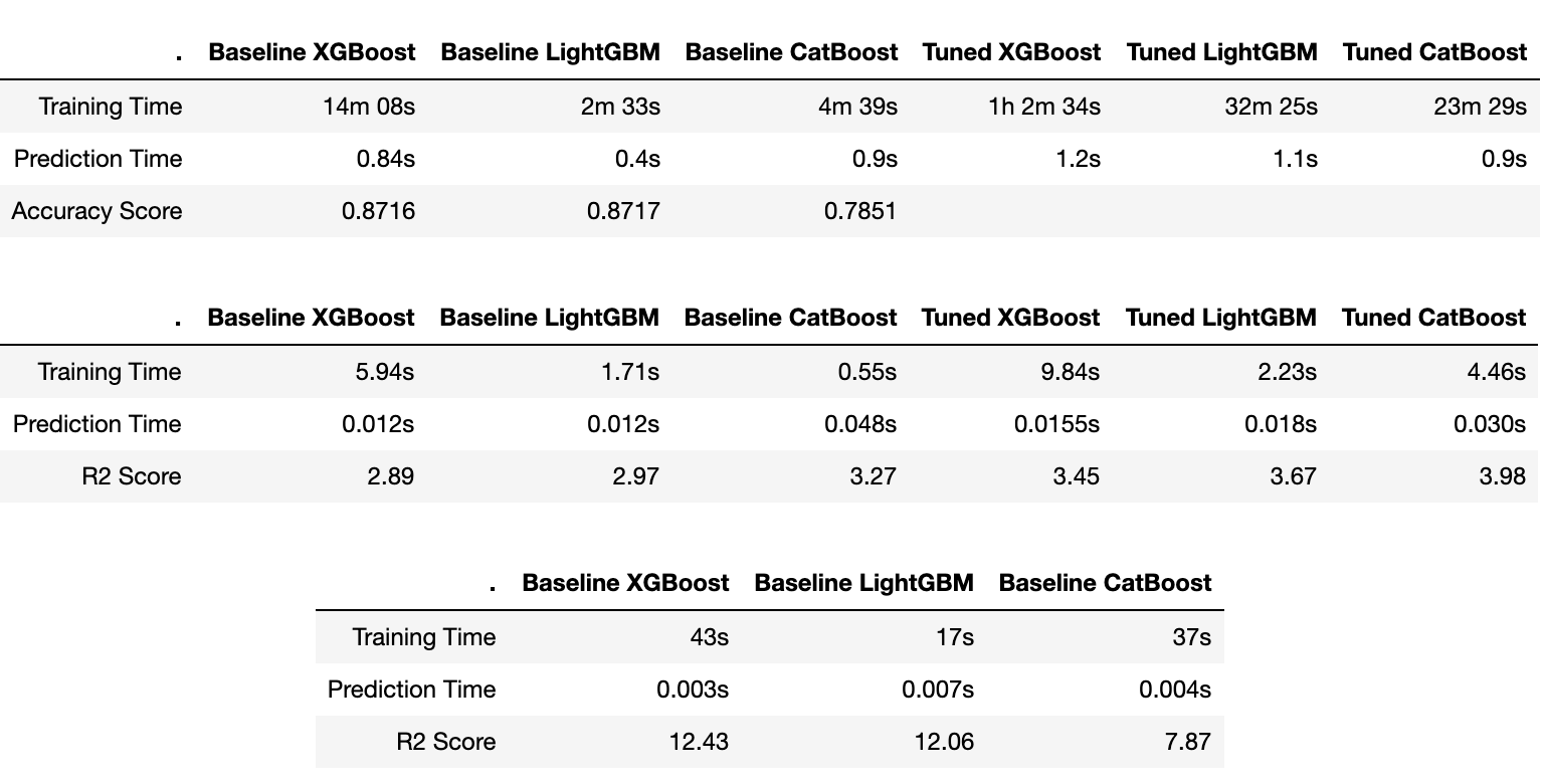
Classification Challenge

Regression Challenge

Massive Dataset Challenge

2. Interpretability

A model’s prediction score only paints a partial picture of its predictions. We also want to know why the model is making its predictions.

Here we plot the model’s feature importances, SHAP values and draw an actual decision tree to get a firmer understanding of the model’s predictions.

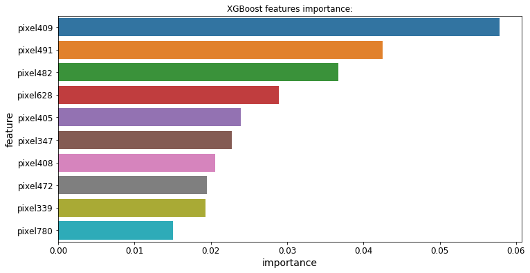
Feature Importance

All 3 boosting models offer a .feature_importances_ attribute that allows us to see which features influence each model’s predictions the most:

Classification Challenge

Regression Challenge

Massive Dataset Challenge

SHAP Values

Another way to get an overview of the distribution of the impact each feature has on the model output is the SHAP summary plot. SHAP values are fair allocation of credit among features and have theoretical guarantees around consistency from game theory which makes them generally more trustworthy than typical feature importances for the whole dataset.

Classification Challenge

Regression Challenge

Plot the Trees

Finally, XGBoost and LightGBM allow us to draw out the actual decision trees used to make predictions, which is excellent for getting a better intuition about each feature’s prediction power on the target variable.

CatBoost ships with no plotting function for its trees. If you really want to visualize CatBoost results, a work-around is proposed here: https://blog.csdn.net/l_xzmy/article/details/81532281

Classification Challenge

Regression Challenge

Model Comparison

Overview

• If you want to dive deeper into these algorithms, here are the links to papers that introduced them:
  • CatBoost: gradient boosting with categorical features support
  • LightGBM: A Highly Efficient Gradient Boosting Decision Tree
  • XGBoost: A Scalable Tree Boosting System

CatBoost

• Offers significantly better accuracy and training times than XGBoost
• Supports categorical features out of the box so we don’t need to preprocess categorical features (for example by LabelEncoding or OneHotEncoding them). In fact, the CatBoost documentation specifically warns against using one-hot encoding during preprocessing as “this affects both the training speed and the resulting quality”.
• Is better at handling overfitting, specially on small datasets by implementing ordered boosting
• Supports out-of-the-box GPU training (just set task_type = “GPU”)
• Handles missing values out of the box

LightGBM

• Offers significantly better accuracy and training times than XGBoost
• Supports parallel tree boosting and offers much better training speeds even on large datasets (than XGBoost).
• Achieves blazing fast training speeds and lower memory usage by using a histogram-esque algorithm which buckets continuous features into discrete ones.
• Achieves great accuracy by using leaf-wise split instead of level-wise split which results in converging very quickly and in very complex trees that can capture the underlying patterns of the training data. Use num_leaves and max_depth hyper-parameters to control for overfitting.

XGBoost

• Supports parallel tree boosting
• Uses regularization to contain overfitting
• Supports user-defined evaluation metrics
• Handles missing values out of the box
• Is much faster than traditional gradient boosting methods like AdaBoost

The Hyperparameters

Checkout the documentations below for a full list of hyper-parameters for these models:

• XGBoost Parameters
• LightGBM Parameters
• CatBoost Parameters

Let’s take a look at the most important parameters of each model!

Catboost

n_estimators — The maximum number of trees that can be built.

learning_rate — The learning rate. Used for reducing the gradient step.

eval_metric — The metric used for overfitting detection and best model selection.

depth — Depth of the tree.

subsample — Sample rate of rows, can’t be used in a Bayesian boosting type setting.

l2_leaf_reg — Coefficient at the L2 regularization term of the cost function.

random_strength — The amount of randomness to use for scoring splits when the tree structure is selected. Use this parameter to avoid overfitting the model.

min_data_in_leaf — The minimum number of training samples in a leaf. CatBoost does not search for new splits in leaves with samples count less than the specified value.

colsample_bylevel, colsample_bytree, colsample_bynode— Rate of sampling of columns at the levels, trees and nodes respectively.

task_type — Takes in values “GPU” or “CPU”. If the dataset is large enough (starting from tens of thousands of objects), training on GPU gives a significant speedup compared to training on CPU. The larger the dataset, the more significant is the speedup.

boosting_type — By default, the boosting type is set to “Ordered” for small datasets. This prevents overfitting but it is expensive in terms of computation. Try to set the value of this parameter to “Plain” to speed up the training.

rsm — For datasets with hundreds of features this parameter speeds up the training and usually does not affect the quality. It is not recommended to change the default value of this parameter for datasets with few (10-20) features.

border_count — This parameter defines the number of splits considered for each feature. By default, it is set to 254 (if training is performed on CPU) or 128 (if training is performed on GPU).

LightGBM

num_leaves — Maximum number of leaves in a tree. In LightGBM num_leaves must be set lesser than 2^(max_depth), to prevent overfitting. Higher values result in increased accuracy but maybe prone to overfitting.

max_depth — Max depth the tree can grow to. Helpful in preventing overfitting.

min_data_in_leaf — Minimum data in each leaf. A small value maybe cause overfitting.

eval_metric — The metric used for overfitting detection and best model selection.

learning_rate — The learning rate. Used for reducing the gradient step.

n_estimators — The maximum number of trees that can be built.

colsample_bylevel, colsample_bytree, colsample_bynode— Rate of sampling of columns at the levels, trees and nodes respectively.

boosting_type — Accepts the following values:

• ‘gbdt’, traditional Gradient Boosting Decision Tree.
• ‘dart’, Dropouts meet Multiple Additive Regression Trees.
• ‘goss’, Gradient-based One-Side Sampling.
• ‘rf’, Random Forest.

n_jobs — Number of parallel threads. Use -1 to use all available threads.

min_split_again — Minimum loss reduction required to make a further partition on a leaf node of the tree.

feature_fraction — Fraction of features used at each iteration. Set this value lower to increase training speeds.

bagging_fraction — Fraction of data used at each iteration. Set this value lower to increase training speeds.

application — default=regression, type=enum, options=

• regression : perform regression task
• binary : Binary classification
• multiclass: Multiclass Classification
• lambdarank : lambdarank application

num_iterations — Iterations of boosting iterations to perform.

max_bin — Maximum number of bins used to bucket feature values. Useful to prevent overfitting.

That’s it!

I hope you found this analysis useful!

Once again, you can find the accompanying code here. I encourage you to fork the kernel, and play with the code. Happy Experimenting!