I’ve recently been having a lot of fun playing with CERN’s Large Hadron Collider datasets, and I thought I’ll share some of the things I’ve learnt along the way. The 2 main things I’ll be exploring in this post are:

1. Particle identification: training a classifier to detect electrons, protons, muons, kaons and pions
2. Searching for dark matter: training a classifier to distinguish between background noise and the signal, and then applying clustering algorithms to find potential traces of dark matter interaction in this signal

You can find the complete code as a Kaggle kernel here. I encourage you to fork it and mess around with it! You can find more LHC datasets to play with here. Disclaimer: I’m not a particle physicist. I’m simply a machine learning engineer who loves playing with interesting datasets.

Table of Contents

1. Particle Physics and the Standard Model
2. Behind the curtains of the Large Hadron Collider
3. Machine Learning Challenges
4. Particle Identification
   1. The Sub-Detectors
      1. Tracking system
      2. Ring-Imaging Cherenkov detector
      3. Electromagnetic and hadron calorimeters
      4. Muon chamber
   2. A Uniform Dependency Curve
      1. Boosting: AdaBoost classifier with a modified loss function modification
      2. Neural Network: An adversarial neural network combined with a standard neural network to prevent non-flatness of the classifier
5. Searching for dark matter
   1. The Challenge
   2. So what might a dark matter signal look like?
   3. Eliminating Background
   4. Looking for signal in the dataset
      1. Using an XGBoost classifier to separate signal from background
      2. Using DBSCAN to find signal clusters
6. Looking ahead to SHiP

Particle Physics and the Standard Model

Let’s start with a super quick intro to particle physics and the Standard Model. 

The Standard Model describes what the universe is made up of and how it holds together. It has 2 central ideas:

1. All matter is made up of particles.
2. These particles interact with each other by exchanging other particles associated with the fundamental forces.

The essential grains of matter are fermions, and the essential force carriers are bosons.

Fermions

The 12 fermions are the building blocks of matter. They come in 2 families:

• Lepton are a group of 6 particles, with electrons being the best known.
• Quarks are also a group of 6 particles, the most interesting of which are the up and down quarks which organize together to make protons and neutrons. Unlike the electrons, protons and neutrons aren’t actually fundamental particles. Protons are made up of 2 up quarks and 1 down quark; while the neutrons are made up of 2 down quarks and 1 up quark.
In addition, quarks combine together to make up Hadrons. There are 2 kinds of Hadrons:
• Baryon
  • made up of 3 quarks
• Mesons
  • made up of 2 quarks (quark and anti-quark)

Bosons

Fermions interact with each other through fundamental forces, and bosons are the building blocks of these forces. Each force comes with one or more force carriers:

• Strong force:
  • gluon – strong force carried by gluons binds the quarks within protons and neutrons
  • photon – carries electromagnetic force
• Weak force, very short range – Weak interactions are a million times weaker than the strong interaction
  • Carried by Z and W bosons – the weak force is responsible for radioactive decay.
  • Higgs boson explains the presence of unexplained mass in some particles.

Pretty much everything we see in the universe is made of up quarks, down quarks and electrons. All the other things exist only for a short amount of time before decaying into other particles.

Here’s a video that goes into more detail about the standard model if you’re curious.

Behind the curtains of the Large Hadron Collider

Next, let’s take a quick tour of how the LHC works!

LHC is a 16 mile tunnel, surrounded by 4 big detectors – ALICE, ATLAS, CMS and LHCb. It orchestrates 40 million bunch collisions per second and produces 10 petabytes of data per year!

The LHC Cycle

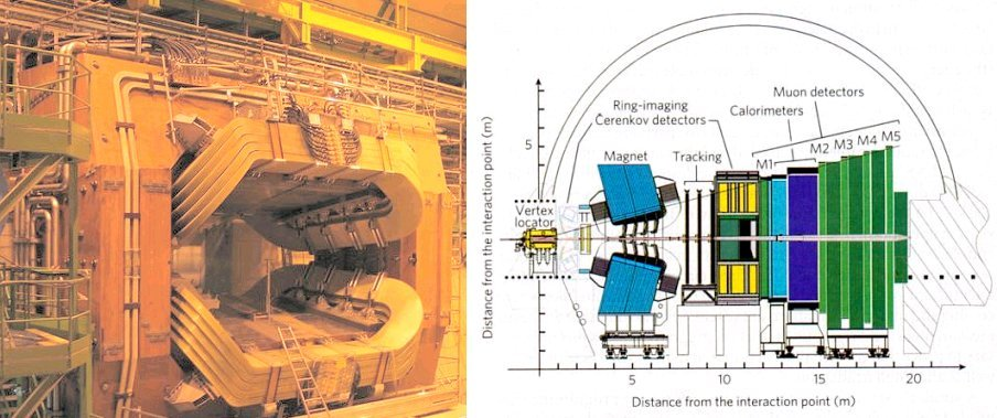
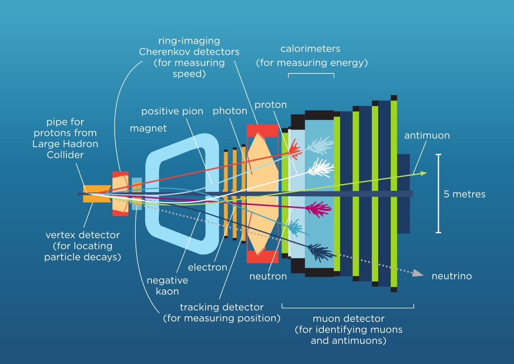
LHC experiments have an absolutely fascinating lifecycle! The LHC starts by creating protons out of hydrogen atoms, and then accelerating them to almost the speed of light (0.9999999c). It then groups these protons into bunches of about 100 billion protons each and smashes them into each other. The proton-proton collisions produce a lot of other particles that decay into other particles. The detector (which is essentially a sub-atomic digital camera surrounding the collision) measures the energy and momentum of every particle flying out of the collision event. Once this data is collected, an algorithm tries to reconstruct the parameters of trajectories of different particles, and identify the types of those particles by calculating their mass.

Every particle leaves different traces in different sub-detectors of the experiment. For example, electrons leave tracks at tracking system and electromagnetic calorimeter. Photons leave no traces in tracking system but leave traces in the electromagnetic calorimeter. Hadrons like protons, kaons, and pions leave tracks in inner most tracking system and electromagnetic calorimeter and hadronic calorimeter. Finally, muons, the slightly heavier cousins of electrons fly through the whole detector and leave traces everywhere.

Once the individual trajectories of all the particles have been reconstructed, they’re combined into vertices and we get a map of the whole event. Most of this data is discarded and special selection procedures called triggers are used to weed out only particularly interesting events for further analysis. The design of these triggers is an interesting ML problem.

If you want to explore how the LHC works further, here’s a great video from CERN:

Also, here’s a breath-taking simulation of LHCb’s output that I really encourage you to check out.

Alright, now we’re ready to start experimenting with some machine learning!

Machine Learning Challenges

A few of the ML challenges in particle physics are:

• Precise and fast particle tracking (single tracks, shower, jets etc.)
• Particle Identification
• Fast and accurate data processing, and design of triggers
• Anomaly detection (data quality and infrastructure monitoring)
• Detector design optimization (using bayesian optimization, surrogate modeling etc.)

In this post, I’ll be exploring particle identification (training a classifier to detect electrons, protons, muons, kaons and pions) and dark matter detection (training a classifier to distinguish between background noise and the signal, and then applying clustering algorithms to find potential traces of dark matter in this signal).

Let’s begin!

Particle Identification

The goal of particle identification is to identify the type of a particle associated with a track using responses from different detector systems.

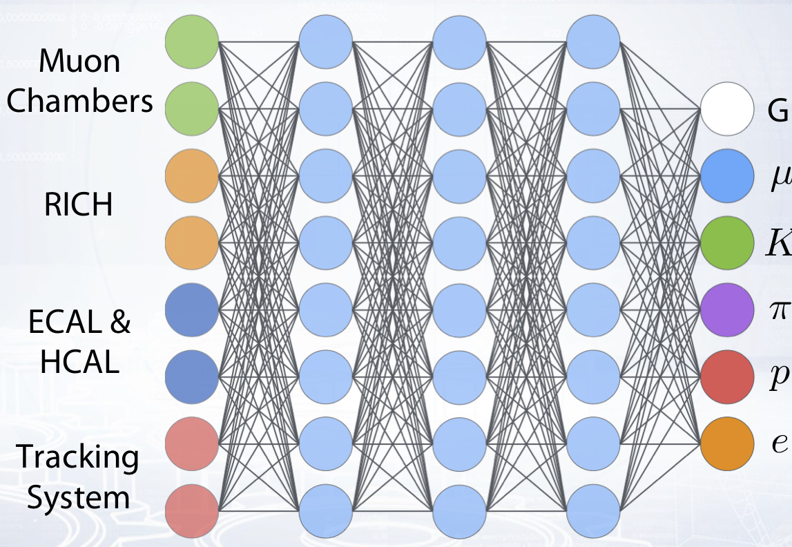
Particle identification is a multi-classification problem in machine learning. There are five particle types: Electron, Proton, Kaon, Pion and Muon.

There are also five different detector systems: Tracking system, Ring Imaging Cherenkov detector, Electromagnetic calorimeter and Hadron calorimeter and finally Muon Chambers.

The inputs to the classifier are the particle track responses in the various sub-detector systems.

• For example, tracking systems measure information about particle track parameters, track fit quality, particle momentum and charge, and also decay vertex coordinates.
• RICH detector measures the particle emission angle or delta likelihood for a different particle type hypotheses or quality of circles fit in the detector.
• Calorimeters measure a particle energy and number of responses for these particles.
• The Muon system detects if a track hits the Muon chamber, and how much active chambers correspond to the track.

Outputs of the classifier are six labels, five of them correspond to five different particle types and Ghost is a catch-all for noisy tracks and other particle types.

Modern detectors in high energy physics (including the one I was able to train) achieve an area under the ROC curve in the range from 0.9 to 0.995 depending on particle type.

Each particle has a certain energy, momentum and mass. Energy and momentum are determined by the speed of the particle, and mass by its type. From the law of conservation of energy we know that when a particle decays, the energy of the mother particle = the sum of energy of the particles it decays into.

From the law of conservation of momentum we know that when a particle decays, the momentum of the mother particle = the vector sum of momentum of the particles it decays into.

Therefore, we can determine the mass of the mother particle using the masses, energy and momentum of the daughter particles. The trajectories of the daughter particles also allow us to determine the angle between them and thus ensure that they originate from the same mother particle.

The various sub-detectors help estimate a particle’s trajectory, momentum, energy and type to be able to recognize particle decays and reconstruct mother particle’s parameters (for e.g. the mass).

The Sub-Detectors

The inside of a detector is a fascinating place. There are 5 sub-detectors:

1. The tracking system recognizes a particle’s trajectory aka its track, estimates parameters of this trajectory, and measures the particle momentum.
2. The Ring-Imaging Cherenkov detector is responsible for the particle type identification, using momentum measured in the tracking system and its emission angle estimated in the RICH detector.
   1. The RICH detector registers photons emitted by particles.
   2. Machine learning algorithms can be used to build clusters of photons (orange dots) and track positions (blue dots) and to identify a particle type in the RICH detector.
      
3. Electromagnetic and hadron calorimeters measure particle energies. Particles interact with the matter of the calorimeter and lose their energy. The calorimeter measures how much energy the particles lose before they stop. Calorimeters are located after the tracking system and RICH detector, because they stop all particles except muons and neutrinos.
   1. A single particle can activate several crystals of the calorimeter. Machine learning algorithms can be used to recognize clusters of these crystals activated by each particle and estimate the particle energy more accurately.
   2. Photons also create clusters in the calorimeter, but they leave no traces in the tracking system and their tracks are not recognized. ML can be used to recognize clusters of photons and separate them from clusters of electrons, or just noise clusters.
      
4. Muon chamber detects muons and also estimates their energy. It is the last and the heaviest system of a detector because muons weakly interact with matter and leave almost no response in the calorimeters. A particle track (measured in the tracking system) is extrapolated into the muon system and if the track passes through active muon chambers, the particle is essentially labelled a muon.
   1. Machine learning can help recognize active chambers for tracks and distinguish them from noise chambers thereby improving the quality of muon identification.
   2. If you want to dive deeper, this is a good place to start: http://cds.cern.ch/record/1495721/files/epjc.73.2431.pdf

A Uniform Dependency Curve

The quality of the particle identification depends on particle parameters such as momentum, transverse momentum or energy. If the quality of classification significantly drops in areas of low and high momentum or energy (as is the case in the graph below), our model can become unreliable.

In an ideal world, we’d like to have no such aberrations in dependencies, and have a flat or uniform dependency curve between particle identification quality and the different particle parameters.

To get flatter signal efficiency on particle momentum we can try 2 models:

1. Boosting: AdaBoost classifier with a modified loss function modification

from sklearn.ensemble import AdaBoostClassifier
from sklearn.tree import DecisionTreeClassifier

clf = AdaBoostClassifier(n_estimators=100, learning_rate=0.01, random_state=42,
								base_estimator=DecisionTreeClassifier(max_depth=6,
												min_samples_leaf=30, random_state=42))
clf.fit(training_data[features].values, training_data.Class.values)
proba_clf = clf.predict_proba(validation_data[features].values)
log_loss(validation_data.Class.values, proba_clf)

I won’t go into too much detail about how to implement this here, but if you’re curious, you can read this paper by Alex M. Rogozhnikov and this one by Denis Derkach. In summary, we modify the AdaBoost loss function to:

2. Neural Network: An adversarial neural network combined with a standard neural network to prevent non-flatness of the classifier

from keras.layers.core import Dense, Activation
from keras.models import Sequential
from keras.optimizers import Adam
from keras.utils import np_utils
def nn_model(input_dim):
    model = Sequential()
    model.add(Dense(100, input_dim=input_dim))
    model.add(Activation('tanh'))

    model.add(Dense(6))
    model.add(Activation('softmax'))

    model.compile(loss='categorical_crossentropy', optimizer=Adam())
    return model

nn = nn_model(len(features))
nn.fit(training_data[features].values, np_utils.to_categorical(training_data.Class.values), verbose=1, nb_epoch=5, batch_size=256)

# predict each track
proba_nn = nn.predict_proba(validation_data[features].values)
log_loss(validation_data.Class.values, proba_nn)

We first train a regular neural network classifier to identify the particle type without any special modifications of its loss function. Then we train an adversary network (with a loss function like categorical cross-entropy) which takes in the particle classifier outputs as inputs, and predicts a particle’s parameters such as momentum or mass.

The de-correlated network shows a much flatter dependency on its output than just a traditional neural network without adversary.

If you’re interested in diving deeper, this paper is a good starting point.

For me, the AdaBoost model ended up performing slightly better than the neural network in this case. Here’s a plot of the ROC curves for all particle classifiers.

plt.figure(figsize=(9, 6))
u_labels = numpy.unique(labels)
for lab in u_labels:
     y_true = labels == lab
     y_pred = predictions[:, lab]
     fpr, tpr, _ = roc_curve(y_true, y_pred)
     auc = roc_auc_score(y_true, y_pred)
     plt.plot(tpr, 1-fpr, linewidth=3, label=class_label_correspondence[lab] + ', AUC = ' + str(numpy.round(auc, 4)))
     plt.xlabel('Signal efficiency (TPR)', size=15)
     plt.ylabel("Background rejection (1 - FPR)", size=15)
     plt.xticks(size=15)
     plt.yticks(size=15)
     plt.xlim(0., 1)
     plt.ylim(0., 1)
     plt.legend(loc='lower left', fontsize=15)
     plt.title('One particle vs rest ROC curves', loc='right', size=15)
     plt.grid(b=1)

Also, the AdaBoost classifier achieved a fairly uniform curve of signal efficiency dependence for Muons on momentum.

sel = spectator < 200 * 10**3
plt.figure(figsize=(5.5*2, 3.5*3))
u_labels = numpy.unique(labels)
    for lab in u_labels:
        y_true = labels == lab
        pred = predictions[y_true, lab]
        spec = spectator[y_true]
        plt.subplot(3, 2, lab+1)
        base_plot(pred, spec, cut=eff, percentile=True, weights=None, n_bins=n_bins, color='1', marker='o', 
                  ms=7, label=class_label_correspondence[lab], fmt='o')
        
        plt.plot([spec.min(), spec.max()], [eff / 100., eff / 100.], label='Global signal efficiecny', color='r', linewidth=3)
        plt.legend(loc='best', fontsize=12)
        plt.xticks(size=12)
        plt.yticks(size=12)
        plt.ylabel('Signal efficiency (TPR)', size=12)
        plt.xlabel(xlabel,size=12)
        plt.ylim(0, 1)
        plt.xlim(spec.min(), spec.max())
        plt.grid(b=1)
plt.tight_layout()

We could tune the parameters further until the slight bump between 25-50 GeV/c and the little dip around 178 GeV/c are normalized.

Onto the next challenge!

Searching for dark matter

Dark matter is a theorized form of matter that potentially might account for approximately 80% of the matter in the Universe, and about a 25% of its total mass-energy.

The Challenge

The 2 primary challenges related to discovery of dark matter are:

• We don’t know what we’re looking for. There are plenty of theories that try to predict presence of dark matter, but we have no inkling of the nature of effect we should be looking for.
• There is no totally clean, observable quantity that we can measure and say yup, this conclusively proves there are traces of dark matter. The direct and indirect targets that might predict dark matter’s presence are laced with noise and background phenomenon that might lead to misleading results.

We’ll try to apply machine learning to tackle the second problem, that of extracting signal that comes from dark matter particle interaction from background noise today!

So what might a dark matter signal look like?

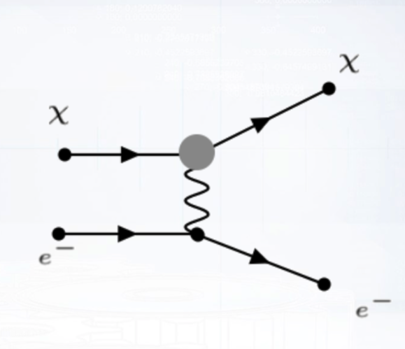Here’s a Feynman diagram of a dark matter particle X scattering an electron of lead nuclei. The boost that the electron gets from this interaction is transferred through the volume of the detector, resulting in an electromagnetic shower. So our goal would be to detect signs of such a shower.

The problem is that when a neutrino interacts with a nucleus, it also produces an electron that get boosted and similar showers are produced, as shown below. This is the background noise we are trying to eliminate.

Eliminating Background

To detect and eliminate this background, we first find these electromagnetic showers. Then classify the signal into background neutrino interaction if:

• neutrino transforms into proton and trajectory of resulting proton is detected (quasi-elastic scattering)
• traces of hadron shower are detected in addition to electromagnetic show (deep inelastic scattering)
• the final particles could possibly be created via dark matter interaction, but the energy-angle correlation of the detected electron points to the presence of neutrino (elastic scattering)

If none of the background interaction conditions above are met, the particle is classified as potentially a dark matter interaction.

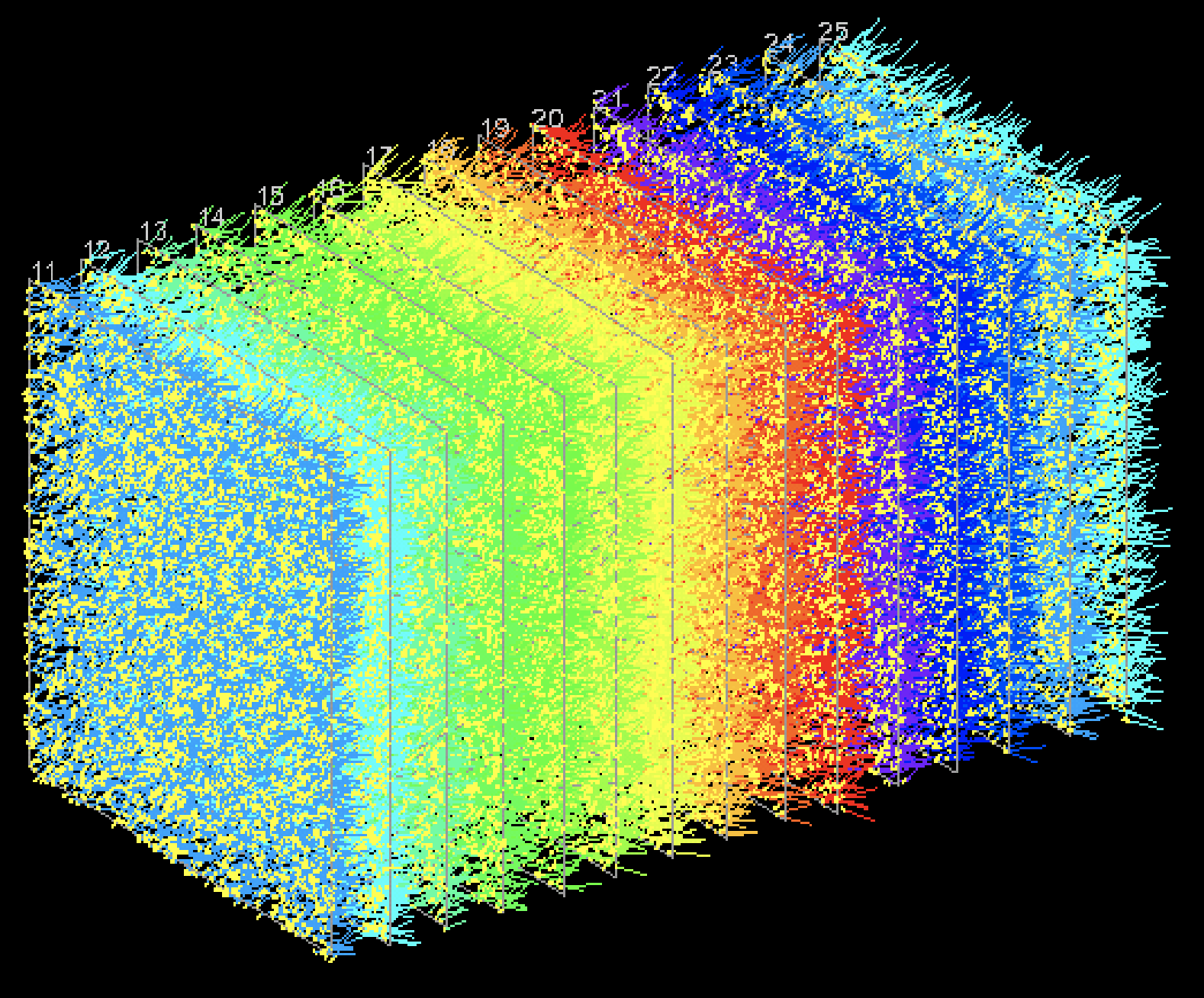
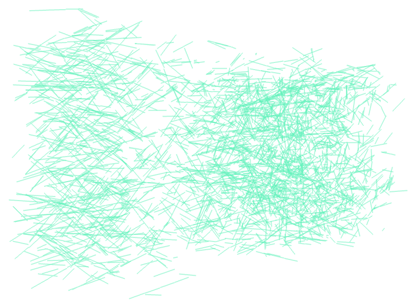
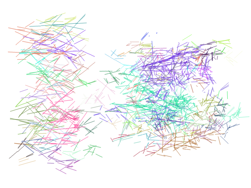
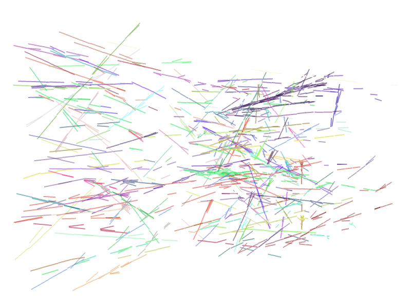
The scale of the problem is massive. In real life experiments, there are approximately 10 million base tracks out of which maybe 1,000 base tracks are results of an electromagnetic shower and the rest are noise. So our goal is to go from the data in the first image, remove background noise to get the second image, then cluster it into potential showers created by dark matter in the third image.

Looking for signal in the dataset

The OPERA dataset is composed of the following features:

• Each base track contains:
  • X, Y, Z co-ordinates
  • angles from origin (TX, TY)
  • goodness of fit of Ag crystals to the base track
• Background consists of base tracks scattered randomly in space, and has a label=0
• Signals consists of base tracks forming a cone shape, has a label=1
• Origin and Energy of shower (X0, Y0, Z0, TX0, TY0, E0)

In addition we compute the following features for every base track:

• distance from the origin (dX, dY, dZ, dTX, dTY)
• alpha, the angle between directions
• d, the projection of base track1

We do this because the most defining characteristic of signal base tracks is that they have a geometric structure – they form tracks (which are just straight lines) and showers, while the background is composed of largely random vectors.

Signal base tracks are also part of a larger vector of movement of particles. This particle moves across many layers in a straight line path. We can look for neighbors (see code below), which are base tracks left by the same particle on adjoining layers. If the base track is the result of a shower, we can find the parent particle by looking for other children particles in the same layer.

def add_neighbours(df, k, metric='minkowski'):
    res = []
    
    for data_ind in tqdm(np.unique(df.data_ind)):
        ind = df.loc[df.data_ind == data_ind].copy()
        ind[['TX', 'TY']] *= 1293
        values = np.unique(ind.Z)
        
        for j in range(1, len(values)):
            z, z_next = (ind.loc[ind.Z == values[j-1]].copy(),
                         ind.loc[ind.Z == values[j]].copy())
            
            b_tree = BallTree(z_next[feat_XY], metric=metric)
            d, i = b_tree.query(z[feat_XY], k=min(k, len(z_next)))
            
            for m in range(i.shape[1]):
                data = z_next.iloc[i[:, m]]
                z_copy = z.copy()
                for col in feat_XY + ['Z']:
                    z_copy[col + '_pair'] = data[col].values
                res.append(z_copy)
            
        res.append(z_next)
        
    res = pd.concat(res)
    for col in feat_XY + ['Z']:
        res['d' + col] = res[col].values - res[col + '_pair'].values
    return res

Using XGBoost to find potential dark matter signals

We are ready to begin estimating the probabilities of selected base tracks being part of the same signal pattern. This is a binary classification problem: is_signal/is_noise. We train an XGboost model on the features generated above, resulting in a baseline ROC of 0.96, precision of ~1.0 and recall of 0.5, which is pret-ty good.

param_grid = {
        'n_estimators':[10, 20], 
        'max_depth':[15],
}

class XGBClassifier_tmp(XGBClassifier):
    def predict(self, X):
        return XGBClassifier.predict_proba(self, X)[:, 1]

clf = GridSearchCV(XGBClassifier_tmp(learning_rate=0.05, subsample=0.8,
                                     colsample_bytree=0.8, n_jobs=20), 
                   param_grid=param_grid, n_jobs=3,
                   scoring='roc_auc',
                   cv=StratifiedKFold(3, shuffle=True, random_state=0),
                   verbose=7)
clf.fit(X_train, y_train)

xgb = XGBClassifier_tmp(base_score=0.5, booster='gbtree', colsample_bylevel=1,
         colsample_bytree=0.8, gamma=0, learning_rate=0.05,
         max_delta_step=0, max_depth=15, min_child_weight=1, missing=None,
         n_estimators=100, nthread=None,
         objective='binary:logistic', random_state=0, reg_alpha=0,
         reg_lambda=1, scale_pos_weight=1, seed=None, silent=True,
         subsample=0.8, n_jobs=24)

prepared_test = add_neighbours(test, k=3)
X_test = prepared_test.drop(['data_ind'], axis=1)
xgb_class.fit(X_train, y_train)
probas = xgb_class.predict(X_test)

We can see below that training the XGBoost model helps tremendously with noise reduction.

Raw Data	After XGBoost

There is one last thing left to do and that is to cluster these base tracks into showers. To cluster this data, we’ll use good ol’ DBSCAN.

Using DBSCAN to find signal clusters

Quick note on the DBSCAN implementation: DBSCAN relies on euclidean distance, which won’t work for our case because we care about relative angles between base tracks, in addition of relative positions.

Just using euclidean distances leads to the following set of clusters. Here DBSCAN just groups tracks placed nearby together, which is no bueno!

To improve the clusters, we simply add an additional term that corresponds to the distance between angles to our distance metric.

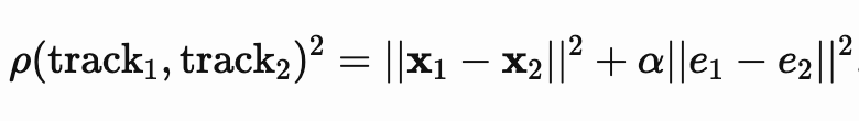
where x is the position (x, y, z) and e is the direction (e1, e2, e3).

from sklearn.cluster import DBSCAN
train.fillna(0, inplace=True)
eps=1.32
min_samples=50
dbscan = cluster.DBSCAN(eps=eps, min_samples=min_samples)
clustering_labels = dbscan.fit_predict(train)

def plot_dataset(dataset, xlim=(-15, 15), ylim=(-15, 15)):
    plt.figure(figsize=figsize)
    plt.scatter(dataset[:,0], dataset[:,1], s=point_size, color="#00B3E9", edgecolor='black', lw=point_border)
    plt.xlim(xlim)
    plt.ylim(ylim)
    plt.show()
    
def plot_clustered_dataset(dataset, y_pred, xlim=(-15, 15), ylim=(-15, 15), neighborhood=False, epsilon=0.5):

    fig, ax = plt.subplots(figsize=figsize)
    
    colors = np.array(list(islice(cycle(['#df8efd', '#78c465', '#ff8e34',
                                     '#f65e97', '#a65628', '#984ea3',
                                     '#999999', '#e41a1c', '#dede00']),
                              int(max(y_pred) + 1))))
    colors = np.append(colors, '#BECBD6')
    
    
    if neighborhood:
        for point in dataset:
            circle1 = plt.Circle(point, epsilon, color='#666666', fill=False, zorder=0, alpha=0.3)
            ax.add_artist(circle1)

    ax.scatter(dataset[:, 0], dataset[:, 1], s=point_size, color=colors[y_pred], zorder=10, edgecolor='black', lw=point_border)
    plt.xlim(xlim)
    plt.ylim(ylim)
    plt.show()
    
def plot_dbscan_grid(dataset, eps_values, min_samples_values):
    
    fig = plt.figure(figsize=(16, 20))
    plt.subplots_adjust(left=.02, right=.98, bottom=0.001, top=.96, wspace=.05,
                        hspace=0.25)


    plot_num = 1

    for i, min_samples in enumerate(min_samples_values):
        for j, eps in enumerate(eps_values):
            ax = fig.add_subplot( len(min_samples_values) , len(eps_values), plot_num)

            dbscan = cluster.DBSCAN(eps=eps, min_samples=min_samples)
            y_pred_2 = dbscan.fit_predict(dataset)

            colors = np.array(list(islice(cycle(['#df8efd', '#78c465', '#ff8e34',
                                                 '#f65e97', '#a65628', '#984ea3',
                                                 '#999999', '#e41a1c', '#dede00']),
                                          int(max(y_pred_2) + 1))))
            colors = np.append(colors, '#BECBD6')


            for point in dataset:
                circle1 = plt.Circle(point, eps, color='#666666', fill=False, zorder=0, alpha=0.3)
                ax.add_artist(circle1)

            ax.text(0, -0.03, 'Epsilon: {} nMin_samples: {}'.format(eps, min_samples), transform=ax.transAxes, fontsize=16, va='top')
            ax.scatter(dataset[:, 0], dataset[:, 1], s=50, color=colors[y_pred_2], zorder=10, edgecolor='black', lw=0.5)


            plt.xticks(())
            plt.yticks(())
            plt.xlim(-14, 5)
            plt.ylim(-12, 7)

            plot_num = plot_num + 1

    plt.show()
plot_clustered_dataset(train, clustering_labels, 
                              xlim=(-14, 5), 
                              ylim=(-12, 7), 
                              neighborhood=True, 
                              epsilon=0.5)
eps_values = [0.3, 0.5, 1, 1.3, 1.5]
min_samples_values = [2, 5, 10, 20, 80]
plot_dbscan_grid(train, eps_values, min_samples_values)

The resulting DBSCAN is able to reconstruct the original particle clusters in the base tracks much better:

I might update this post and the Kaggle kernel with a recurrent neural network in the future. It would be fun to see if we can improve our performance further.

Looking ahead to SHiP

Excellent! From all that background noise, we’ve extracted the signal base tracks that are the best candidates for dark matter particle interactions! w00t!

There is a proposed experiment by CERN called Search for Hidden Particles aka SHiP which is expected to launch in 2025. SHiP is designed more specifically to search for light dark matter and would employ the same techniques we used above to reconstruct dark matter particle trajectories from data. Hopefully, the new data will allow us to determine with greater confidence and accuracy which of these signal clusters are a result of dark matter interactions! When SHiP starts up, I’ll be here ready to dig into the dataset!

If you liked this post, please give the Kaggle kernel an upvote. Thank you!